Footprint representativeness after Chu et al. (2021)

A footprint climatology tells you where the flux came from. This notebook answers the complementary question: how well does that source area stand in for the target area the site is being used to represent? — the model grid cell, the satellite pixel window, or the fixed-radius disc a network product assigns to the tower.

It walks through the whole method of

Chu, H., Luo, X., Ouyang, Z., et al. (2021). Representativeness of Eddy-Covariance flux footprints for areas surrounding AmeriFlux sites. Agricultural and Forest Meteorology 301–302, 108350. doi:10.1016/j.agrformet.2021.108350

in four steps:

1. Build a monthly day/night climatology from half-hourly tower data.

2. Load a land-cover raster and an EVI stack onto the footprint grid.

3. Run ``assess_representativeness`` — the geometry metrics of Eqs. 1–3 and the categorical and continuous evaluations of Sect. 2.4.

4. Produce the four figures of representativeness_plotting.

The theory, all seven equations, and the classification tables are on the Footprint representativeness page. The validation page compares these metrics against the authors’ own published values.

The tower record is the bundled AmeriFlux US-CRT BASE file (Curtice Walter-Berger cropland, north-west Ohio), May–October 2011.

import tempfile
from pathlib import Path

import matplotlib.pyplot as plt
import numpy as np
import pandas as pd
import rasterio
import xarray as xr
from matplotlib.colors import BoundaryNorm, ListedColormap
from pyproj import Transformer
from rasterio.transform import from_origin

from fluxfootprints import (
    ASYMMETRY_THRESHOLD,
    BIAS_THRESHOLD,
    assess_representativeness,
    build_climatology,
    compute_aerodynamic_params,
    evaluate_landcover,
    load_amf_df,
    load_config,
    monthly_climatologies,
    plot_bias_density,
    plot_footprint_target_scatter,
    plot_landcover_composition,
    plot_level_bars,
    representativeness_table,
    sample_raster_on_grid,
)

pd.set_option("display.width", 160)
pd.set_option("display.max_columns", 40)

DATA = Path("..") / ".." / "data"        # repository data/ directory
WORK = Path(tempfile.mkdtemp(prefix="representativeness-"))   # scratch GeoTIFFs

SITE = "US-CRT"
TZ = -5                                   # US-CRT records local standard time
START, END = "2011-05-01", "2011-10-31"   # one growing season
STEP, HALF = 10.0, 1000.0                 # 10 m cells on a +/- 1 km domain
RADII = (100.0, 250.0, 500.0, 1000.0)     # target-area radii [m]

print(f"reading tower data from {DATA.resolve().name}/")

reading tower data from data/

Note on the target radii. Chu et al. (2021) evaluate 250 m to 3000 m (fluxfootprints.TARGET_RADII). US-CRT is a short-canopy cropland site with a 2.5 m tower, so its footprint is only a couple of hundred metres across; a 1 km domain resolves it well and a 3 km disc would tell us nothing the 1 km one does not. The radii above are chosen to bracket this footprint. Pass radii=TARGET_RADII to reproduce the paper’s series.

1. Build a monthly day/night climatology

Chu et al. aggregate every half-hourly footprint of a calendar month into a daytime and a nighttime climatology, truncate each at the contour enclosing 80 % of the source weight, and rescale the retained cells to sum to one. That truncated climatology is the unit of analysis for everything downstream.

First the tower record. load_config reads the site’s .ini, load_amf_df reads the AmeriFlux BASE file, and the columns are renamed to the solver’s names.

config = load_config(DATA / "US-CRT_config.ini")
lat = float(config["station_latitude"])
lon = float(config["station_longitude"])
print(f"{SITE}: {lat:.4f} N, {lon:.4f} E")

frame = load_amf_df(DATA / "AMF_US-CRT_BASE_HH_3-5.csv", config).rename(
    columns={
        "WD": "wind_dir",
        "WS": "umean",
        "USTAR": "ustar",
        "MO_LENGTH": "ol",
        "V_SIGMA": "sigmav",
    }
)

season = frame.loc[START:END, ["wind_dir", "umean", "ustar", "ol", "sigmav"]].dropna()
# Kljun et al. (2015) do not apply in very weak turbulence; the paper filters
# those half-hours out before aggregating (its Table S2).
season = season[season["ustar"] >= 0.15]
season = compute_aerodynamic_params(
    season, inst_height=2.5, crop_height=0.4, veg_type="alfalfa"
)
print(f"{len(season)} half-hours from {season.index.min()} to {season.index.max()}")
season.head()

US-CRT: 41.6285 N, -83.3471 E
5158 half-hours from 2011-05-02 20:00:00 to 2011-10-31 17:30:00

	wind_dir	umean	ustar	ol	sigmav	zm	z0
TIMESTAMP_START
2011-05-02 20:00:00	267.2680	2.18254	0.16236	27.346434	0.48027	2.232	0.0492
2011-05-03 05:00:00	37.9146	2.49536	0.15085	58.736718	0.66084	2.232	0.0492
2011-05-03 05:30:00	59.4592	4.49470	0.27739	686.206897	0.73097	2.232	0.0492
2011-05-03 06:00:00	64.3045	3.98159	0.26283	401.209677	0.83509	2.232	0.0492
2011-05-03 06:30:00	56.1142	3.40681	0.22406	354.092527	0.86838	2.232	0.0492

build_climatology runs the Kljun et al. (2015) parameterisation over every half-hour and keeps the per-timestep footprints, which is what the monthly aggregation needs. This takes about a minute at 10 m resolution.

model = build_climatology(
    season,
    model_type="ffp",
    ustar="ustar",
    ol="ol",
    umean="umean",
    sigmav="sigmav",
    wind_dir="wind_dir",
    zm="zm",
    z0="z0",
    h=2000.0,
    dx=STEP,
    dy=STEP,
    domain=(-HALF, HALF, -HALF, HALF),
    verbosity=0,
)

fclim = model.get_footprint_climatology()
captured = float(fclim.sum()) * STEP * STEP
print(fclim.sizes)
print(f"source weight inside the domain: {captured:.1%}")

Frozen({'x': 201, 'y': 201})
source weight inside the domain: 94.3%

The captured fraction matters here more than usual: the truncation fraction is a fraction of the full footprint, not of the captured mass, so a domain holding much less than 80 % of the weight cannot produce a meaningful 80 % contour at all. At 94 % we have room to spare. Note that this is set by resolution as much as by extent — the footprint peaks within tens of metres of a 2.5 m tower, so a coarse grid loses the peak no matter how wide the domain.

Now the aggregation. Day and night are separated at \(SW_{IN,POT} > 0\); monthly_climatologies prefers a precomputed SW_IN_POT column when the record carries one and falls back to solar geometry otherwise, which is why it wants the tower position and the time zone.

clim = monthly_climatologies(
    model,
    partition="month+daynight",
    latitude=lat,
    longitude=lon,
    tz=TZ,
)
clim

<xarray.Dataset> Size: 4MB
Dimensions:                (month: 6, period: 2, x: 201, y: 201)
Coordinates:
  * month                  (month) datetime64[ns] 48B 2011-05-01 ... 2011-10-01
  * period                 (period) <U9 72B 'daytime' 'nighttime'
  * x                      (x) float64 2kB -1e+03 -990.0 -980.0 ... 990.0 1e+03
  * y                      (y) float64 2kB -1e+03 -990.0 -980.0 ... 990.0 1e+03
Data variables:
    footprint_climatology  (month, period, x, y) float64 4MB 0.0 0.0 ... 0.0 0.0
    n_times                (month, period) int64 96B 591 214 727 ... 347 509 297
    contour_level          (month, period) float64 96B 4.949e-06 ... 4.877e-06
    contour_n_cells        (month, period) int64 96B 154 130 158 ... 157 214 160
Attributes:
    partition:         month+daynight
    contour_fraction:  0.8
    min_times:         1
    n_timesteps:       5158
    description:       Monthly footprint climatologies truncated at the 80% s...
    reference:         Chu, H., et al. (2021). Agric. For. Meteorol., 301-302...

xarray.Dataset

• Dimensions:
  • month: 6
  • period: 2
  • x: 201
  • y: 201
• Coordinates: (4)
  • month
    (month)
    datetime64[ns]
    2011-05-01 ... 2011-10-01

    array(['2011-05-01T00:00:00.000000000', '2011-06-01T00:00:00.000000000',
           '2011-07-01T00:00:00.000000000', '2011-08-01T00:00:00.000000000',
           '2011-09-01T00:00:00.000000000', '2011-10-01T00:00:00.000000000'],
          dtype='datetime64[ns]')

  • period
    (period)
    <U9
    'daytime' 'nighttime'

    array(['daytime', 'nighttime'], dtype='<U9')

  • x
    (x)
    float64
    -1e+03 -990.0 ... 990.0 1e+03

    array([-1000.,  -990.,  -980., ...,   980.,   990.,  1000.], shape=(201,))

  • y
    (y)
    float64
    -1e+03 -990.0 ... 990.0 1e+03

    array([-1000.,  -990.,  -980., ...,   980.,   990.,  1000.], shape=(201,))

• Data variables: (4)
  • footprint_climatology
    (month, period, x, y)
    float64
    0.0 0.0 0.0 0.0 ... 0.0 0.0 0.0 0.0

    units :

    1

    long_name :

    renormalised footprint climatology

    contour_fraction :

    0.8

    array([[[[0., 0., 0., ..., 0., 0., 0.],
             [0., 0., 0., ..., 0., 0., 0.],
             [0., 0., 0., ..., 0., 0., 0.],
             ...,
             [0., 0., 0., ..., 0., 0., 0.],
             [0., 0., 0., ..., 0., 0., 0.],
             [0., 0., 0., ..., 0., 0., 0.]],
    
            [[0., 0., 0., ..., 0., 0., 0.],
             [0., 0., 0., ..., 0., 0., 0.],
             [0., 0., 0., ..., 0., 0., 0.],
             ...,
             [0., 0., 0., ..., 0., 0., 0.],
             [0., 0., 0., ..., 0., 0., 0.],
             [0., 0., 0., ..., 0., 0., 0.]]],
    
    
           [[[0., 0., 0., ..., 0., 0., 0.],
             [0., 0., 0., ..., 0., 0., 0.],
             [0., 0., 0., ..., 0., 0., 0.],
    ...
             [0., 0., 0., ..., 0., 0., 0.],
             [0., 0., 0., ..., 0., 0., 0.],
             [0., 0., 0., ..., 0., 0., 0.]]],
    
    
           [[[0., 0., 0., ..., 0., 0., 0.],
             [0., 0., 0., ..., 0., 0., 0.],
             [0., 0., 0., ..., 0., 0., 0.],
             ...,
             [0., 0., 0., ..., 0., 0., 0.],
             [0., 0., 0., ..., 0., 0., 0.],
             [0., 0., 0., ..., 0., 0., 0.]],
    
            [[0., 0., 0., ..., 0., 0., 0.],
             [0., 0., 0., ..., 0., 0., 0.],
             [0., 0., 0., ..., 0., 0., 0.],
             ...,
             [0., 0., 0., ..., 0., 0., 0.],
             [0., 0., 0., ..., 0., 0., 0.],
             [0., 0., 0., ..., 0., 0., 0.]]]], shape=(6, 2, 201, 201))

  • n_times
    (month, period)
    int64
    591 214 727 162 ... 608 347 509 297

    long_name :

    contributing timesteps

    array([[591, 214],
           [727, 162],
           [713, 157],
           [646, 187],
           [608, 347],
           [509, 297]])

  • contour_level
    (month, period)
    float64
    4.949e-06 7.234e-06 ... 4.877e-06

    units :

    m-2

    long_name :

    source weight at the contour

    array([[4.94931543e-06, 7.23372297e-06],
           [4.81165151e-06, 6.63963404e-06],
           [4.27392540e-06, 5.58384255e-06],
           [4.03031790e-06, 5.72514281e-06],
           [2.96156894e-06, 5.28603576e-06],
           [2.99356499e-06, 4.87718694e-06]])

  • contour_n_cells
    (month, period)
    int64
    154 130 158 128 ... 218 157 214 160

    long_name :

    cells inside the contour

    array([[154, 130],
           [158, 128],
           [172, 151],
           [180, 150],
           [218, 157],
           [214, 160]])

• Attributes: (6)

  partition :

  month+daynight

  contour_fraction :

  0.8

  min_times :

  1

  n_timesteps :

  5158

  description :

  Monthly footprint climatologies truncated at the 80% source-weight contour and renormalised to unit sum, after Chu et al. (2021), Sect. 2.2.

  reference :

  Chu, H., et al. (2021). Agric. For. Meteorol., 301-302, 108350.

# Half-hours contributing to each monthly climatology
clim.n_times.to_pandas()

period	daytime	nighttime
month
2011-05-01	591	214
2011-06-01	727	162
2011-07-01	713	157
2011-08-01	646	187
2011-09-01	608	347
2011-10-01	509	297

Six months, split day and night: twelve climatologies, each already truncated at its own 80 % contour and renormalised. contour_n_cells shows how compact they are — 130 to 220 cells of 10 m, so a source area of one to two hectares.

clim.contour_n_cells.to_pandas()

period	daytime	nighttime
month
2011-05-01	154	130
2011-06-01	158	128
2011-07-01	172	151
2011-08-01	180	150
2011-09-01	218	157
2011-10-01	214	160

2. Load a land-cover raster and an EVI stack

The evaluations of Sect. 2.4 compare the climatology against two external products: a categorical land-cover map, and a time series of a continuous vegetation index.

In production, fluxfootprints.representativeness_data fetches both straight from Google Earth Engine onto a tower-centred grid — NLCD for the categorical field, and Landsat 5/8 Collection 2 EVI (the paper’s Eq. 4, cloud-screened to < 1 % obscured) for the continuous one:

from fluxfootprints import fetch_landsat_evi, fetch_nlcd, footprint_grid_geometry

geom = footprint_grid_geometry(model.x, model.y, lat, lon)

nlcd = fetch_nlcd(geom.x_origin, geom.y_origin, geom.crs, year=2016)
scenes = fetch_landsat_evi(
    geom.x_origin, geom.y_origin, geom.crs,
    start="2011-05-01", end="2011-11-01",
)

That needs the gee extra (pip install 'fluxfootprints[gee]') and an authenticated Earth Engine project, so this notebook stays offline and synthesises two stand-in products instead: a 30 m land-cover map and six monthly EVI scenes, written to GeoTIFF exactly as a downloaded product would be. Everything from here on is the real code path.

The landscape is a plausible one for north-west Ohio: the tower stands in a soybean field, with a wooded strip to the south-west, pasture to the north-east, a developed edge to the south-east, and open water to the north.

EPSG = 32617  # WGS 84 / UTM zone 17N, the local zone for US-CRT
east, north = Transformer.from_crs(
    "EPSG:4326", f"EPSG:{EPSG}", always_xy=True
).transform(lon, lat)

RES, N = 30.0, 141                       # 30 m cells, 4.2 km across
half_px = (N // 2) * RES
transform = from_origin(east - half_px - RES / 2, north + half_px + RES / 2, RES, RES)

eastings = (np.arange(N) - N // 2) * RES
northings = (N // 2 - np.arange(N)) * RES
XX, YY = np.meshgrid(eastings, northings)
distance = np.hypot(XX, YY)
bearing = np.degrees(np.arctan2(XX, YY)) % 360.0


def write_geotiff(path, array, dtype, nodata):
    # Write one band to a georeferenced GeoTIFF.
    with rasterio.open(
        path, "w", driver="GTiff", height=N, width=N, count=1,
        dtype=dtype, crs=f"EPSG:{EPSG}", transform=transform, nodata=nodata,
    ) as dst:
        dst.write(array.astype(dtype), 1)


CROPS, FOREST, PASTURE, DEVELOPED, WATER = 82, 41, 81, 21, 11
CLASS_NAMES = {
    82: "Cultivated crops",
    41: "Deciduous forest",
    81: "Hay/pasture",
    21: "Developed, open space",
    11: "Open water",
}

land = np.full((N, N), CROPS, dtype="int16")
land[(distance > 220) & (bearing >= 185) & (bearing < 265)] = FOREST
land[(distance > 320) & (bearing >= 20) & (bearing < 95)] = PASTURE
land[(distance > 700) & (bearing >= 95) & (bearing < 150)] = DEVELOPED
land[(distance > 1300) & ((bearing >= 300) | (bearing < 20))] = WATER

landcover_path = WORK / "US-CRT_landcover_2011.tif"
write_geotiff(landcover_path, land, "int16", 0)

pd.Series(land.ravel()).map(CLASS_NAMES).value_counts(normalize=True).round(3)

Cultivated crops         0.251
Deciduous forest         0.226
Hay/pasture              0.212
Open water               0.157
Developed, open space    0.154
Name: proportion, dtype: float64

The EVI stack gives each class its own seasonal curve. The soybean field swings from bare soil in May to a closed canopy in August and back; the forest and pasture are flatter, and the developed and water classes barely move. That contrast is the whole point: it is what makes a footprint-weighted EVI differ from a disc-averaged one.

PHENOLOGY = {              # EVI by class and month
    CROPS:     {5: 0.16, 6: 0.34, 7: 0.71, 8: 0.78, 9: 0.44, 10: 0.19},
    FOREST:    {5: 0.42, 6: 0.55, 7: 0.58, 8: 0.57, 9: 0.48, 10: 0.32},
    PASTURE:   {5: 0.38, 6: 0.45, 7: 0.41, 8: 0.39, 9: 0.40, 10: 0.33},
    DEVELOPED: {5: 0.15, 6: 0.19, 7: 0.20, 8: 0.20, 9: 0.18, 10: 0.14},
    WATER:     {5: 0.03, 6: 0.03, 7: 0.04, 8: 0.04, 9: 0.03, 10: 0.02},
}

rng = np.random.default_rng(11)
evi_paths = {}
for month in range(5, 11):
    stamp = pd.Timestamp(f"2011-{month:02d}-15")   # one clear scene per month
    field = np.zeros((N, N))
    for code_, curve in PHENOLOGY.items():
        field = np.where(land == code_, curve[month], field)
    field = field + 0.03 * rng.standard_normal((N, N))   # within-class texture
    path = WORK / f"US-CRT_evi_{stamp:%Y%m%d}.tif"
    write_geotiff(path, field, "float32", np.nan)
    evi_paths[stamp] = path

list(evi_paths)

[Timestamp('2011-05-15 00:00:00'),
 Timestamp('2011-06-15 00:00:00'),
 Timestamp('2011-07-15 00:00:00'),
 Timestamp('2011-08-15 00:00:00'),
 Timestamp('2011-09-15 00:00:00'),
 Timestamp('2011-10-15 00:00:00')]

sample_raster_on_grid georeferences the tower-centred footprint grid and warps each raster onto it, so the products line up with the climatology cell for cell. Land-cover codes must go through nearest neighbour — bilinear resampling of class codes invents classes that are not in the legend — which is what categorical=True selects.

landcover = sample_raster_on_grid(
    landcover_path, model.x, model.y, lat, lon, categorical=True
)
scenes = {
    stamp: sample_raster_on_grid(path, model.x, model.y, lat, lon)
    for stamp, path in evi_paths.items()
}

print(landcover.dims, landcover.shape)
print("classes on the grid:", sorted(np.unique(landcover.values[np.isfinite(landcover.values)])))

('x', 'y') (201, 201)
classes on the grid: [np.float64(11.0), np.float64(21.0), np.float64(41.0), np.float64(81.0), np.float64(82.0)]

Before running the analysis, it is worth seeing what the tower actually sees against what the target discs contain.

july_day = clim.footprint_climatology.sel(period="daytime", month="2011-07-01")

codes = sorted(CLASS_NAMES)
cmap = ListedColormap(["#3b6ea5", "#c8b0a0", "#3f7f4f", "#c9d48a", "#d9b45b"])
norm = BoundaryNorm([c - 0.5 for c in codes] + [codes[-1] + 0.5], cmap.N)

fig, axes = plt.subplots(1, 2, figsize=(11, 5), sharex=True, sharey=True)

axes[0].pcolormesh(model.x, model.y, landcover.T, cmap=cmap, norm=norm, shading="auto")
axes[0].set_title("Land cover")

weights = july_day.where(july_day > 0)
mesh = axes[1].pcolormesh(model.x, model.y, weights.T, cmap="magma_r", shading="auto")
fig.colorbar(mesh, ax=axes[1], label="source weight [-]", shrink=0.85)
axes[1].set_title("July 2011 daytime climatology, truncated at 80 %")

for ax in axes:
    for radius in RADII:
        ax.add_patch(plt.Circle((0, 0), radius, fill=False, ec="0.15", lw=0.9, ls="--"))
        ax.annotate(f"{radius:.0f} m", (0, radius), textcoords="offset points",
                    xytext=(3, 3), fontsize=8, color="0.15")
    ax.plot(0, 0, marker="^", ms=9, color="k")
    ax.set_aspect("equal")
    ax.set_xlim(-HALF, HALF)
    ax.set_ylim(-HALF, HALF)
    ax.set_xlabel("east of tower [m]")
axes[0].set_ylabel("north of tower [m]")

handles = [plt.Rectangle((0, 0), 1, 1, fc=cmap(norm(c))) for c in codes]
axes[0].legend(handles, [CLASS_NAMES[c] for c in codes], loc="lower left", fontsize=7.5)
fig.tight_layout()

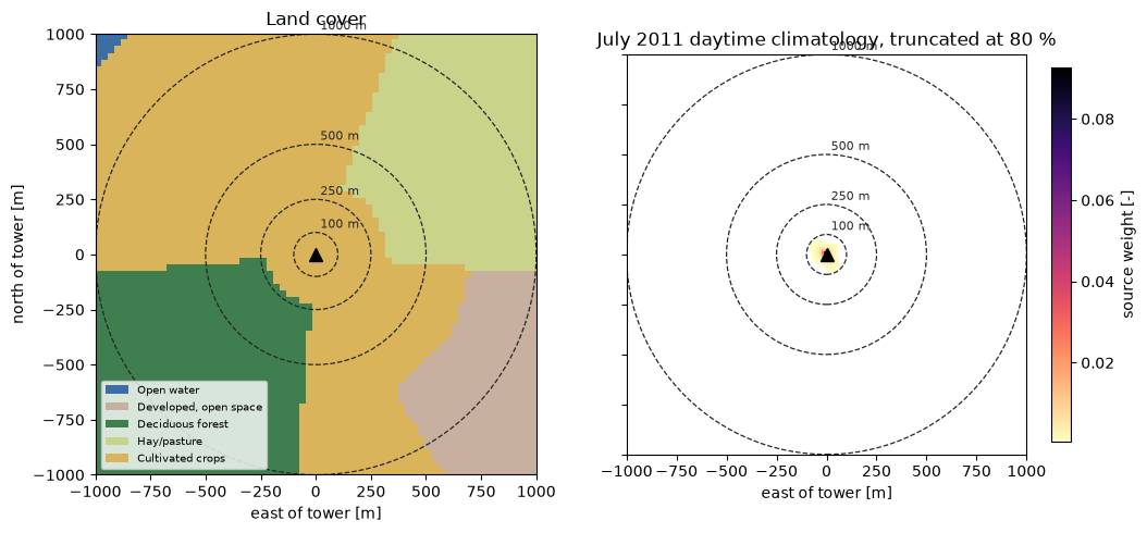
That is the whole problem in one picture. The source area is a compact lobe a couple of hundred metres across, entirely inside the soybean field; the 500 m and 1000 m discs take in forest, pasture, developed ground, and water that the tower never sees.

3. Run assess_representativeness

One call drives everything: the geometry metrics of Eqs. 1–3, the categorical comparison and the continuous one at every radius, and the three-level classification of each. Passing the already-aggregated clim Dataset rather than the model reuses the aggregation instead of repeating it.

results = assess_representativeness(
    clim,
    station_lat=lat,
    station_lon=lon,
    site_id=SITE,
    landcover=landcover,
    continuous=scenes,
    radii=RADII,
    tz=TZ,
)
print(results.shape)
results.reset_index()[["scope", "kind"]].value_counts()

(126, 34)

scope      kind
period     categorical    48
           continuous     48
           climatology    12
site       categorical     8
           continuous      8
site_year  climatology     2
Name: count, dtype: int64

The frame is tidy and sparse: rows of three scopes and three kinds, indexed by (site, year, month, period, radius, variable), with each row carrying only the columns its own analysis produces. Select a slice before reading values off it.

Climatology metrics — Eqs. 1–3

results.query("scope == 'site_year' and kind == 'climatology'").reset_index()[
    ["period", "fetch", "area", "symmetry", "seasonal_overlap", "daynight_overlap"]
].round(3)

	period	fetch	area	symmetry	seasonal_overlap	daynight_overlap
0	daytime	98.873	18266.667	0.597	0.918	0.959
1	nighttime	102.545	14600.000	0.469	0.842	0.959

Reading these:

• X80 ≈ 100 m, A80 ≈ 1.5–1.8 ha. A short canopy on a low tower gives a small source area. The nighttime footprint reaches farther than the daytime one — as the paper finds for > 95 % of its site-years — but here it encloses less area, so nights are the more elongated of the two.

• S80 ≈ 0.60 day, 0.47 night, both comfortably above ASYMMETRY_THRESHOLD (0.30). The wind rose is broad enough that the source area stays roughly disc-like rather than collapsing into a single lobe, though the lower nighttime value reflects exactly the elongation above.

• O80,season ≈ 0.92 day / 0.84 night (Eq. 2). The daytime source area is stable through the season; at night it wanders more, which is the usual signature of light, variable winds under a stable boundary layer.

• O80,daynight ≈ 0.96 (Eq. 3). Day and night sample nearly the same ground here — this site has no drainage flow to send nights somewhere else.

Land-cover representativeness — Sect. 2.4

categorical = results.query("scope == 'site' and kind == 'categorical'").reset_index()
categorical[
    ["period", "radius", "dominant_class", "value_footprint", "value_target",
     "chi2", "p_value", "level"]
].round(3)

	period	radius	dominant_class	value_footprint	value_target	chi2	p_value	level
0	daytime	100.0	82	1.0	1.000	0.000	1.0	high
1	daytime	250.0	82	1.0	0.957	88.851	0.0	low
2	daytime	500.0	82	1.0	0.699	3375.424	0.0	low
3	daytime	1000.0	82	1.0	0.524	28581.048	0.0	low
4	nighttime	100.0	82	1.0	1.000	0.000	1.0	high
5	nighttime	250.0	82	1.0	0.957	88.851	0.0	low
6	nighttime	500.0	82	1.0	0.699	3375.424	0.0	low
7	nighttime	1000.0	82	1.0	0.524	28581.048	0.0	low

The dominant class is cultivated crops (NLCD 82) everywhere, and it holds 100 % of the footprint weight at every radius — the footprint never leaves the field. What changes is the disc: 100 % crop at 100 m, 96 % at 250 m, 70 % at 500 m, and 52 % at 1000 m.

The level column falls to low from 250 m outwards, and it is worth being precise about why. Both shares are still above 80 % at 250 m, so the percentage criteria are met; it is the chi-square test that fails. That test scales both compositions to pseudo-counts by the number of classified cells in the target area — and on a 10 m grid a 250 m disc holds nearly 2000 of them, so even a 4 % difference in composition is resolved as significant. Read the p-value as a comparison against the paper’s fixed 30 m Landsat grid, not as an absolute significance; a finer grid makes the same test stricter. The _composition_chi_square docstring spells this out.

Continuous-field representativeness — Eqs. 5–7

periods = results.query("scope == 'period' and kind == 'continuous'").reset_index()
periods.groupby("radius").agg(
    mean_footprint_evi=("value_footprint", "mean"),
    mean_target_evi=("value_target", "mean"),
    mean_bias=("bias", "mean"),
    within_10pct=("within_threshold", "mean"),
).round(3)

	mean_footprint_evi	mean_target_evi	mean_bias	within_10pct
radius
100.0	0.439	0.437	0.010	1.0
250.0	0.439	0.438	-0.003	1.0
500.0	0.439	0.440	-0.057	0.5
1000.0	0.439	0.419	-0.023	0.333

within_10pct is the share of matched scenes whose sensor location bias (Eq. 6) sits inside BIAS_THRESHOLD (±10 %). It falls from 1.00 at 100 m and 250 m to 0.50 at 500 m and 0.33 at 1000 m: the wider the disc, the less often the tower’s own view of it is within 10 % of the truth. This is the paper’s Sect. 3.3 result, and it comes straight off these rows.

continuous = results.query("scope == 'site' and kind == 'continuous'").reset_index()
continuous[
    ["period", "radius", "slope", "intercept", "r_squared", "p_value", "n",
     "sufficient", "level"]
].round(3)

	period	radius	slope	intercept	r_squared	p_value	n	sufficient	level
0	daytime	100.0	1.014	-0.007	1.000	0.0	6	True	high
1	daytime	250.0	0.989	0.005	0.999	0.0	6	True	high
2	daytime	500.0	0.785	0.096	0.995	0.0	6	True	medium
3	daytime	1000.0	0.628	0.144	0.986	0.0	6	True	medium
4	nighttime	100.0	1.017	-0.009	1.000	0.0	6	True	high
5	nighttime	250.0	0.991	0.003	0.999	0.0	6	True	high
6	nighttime	500.0	0.787	0.095	0.995	0.0	6	True	medium
7	nighttime	1000.0	0.629	0.143	0.986	0.0	6	True	medium

The Eq. 7 model II slope \(\beta_1\) falls from 1.01 at 100 m to 0.63 at 1000 m. A slope below one means the footprint-weighted EVI swings further than the disc average does — the tower tracks its own field’s phenology, while the disc dilutes that swing with forest, pasture, and water that barely change through the season. The classification drops from high to medium as the disc widens, even though \(R^2\) stays above 0.98 throughout: it is the slope leaving the 0.9–1.1 band that costs the site its high.

4. The four figures

fluxfootprints.representativeness_plotting draws the paper’s four diagnostics. Each takes what the analysis functions already return and hands back (fig, ax) without showing or saving anything, so titles, layout, and output stay with the caller.

Fig. 1e — land-cover composition

july_categorical = evaluate_landcover(july_day, landcover, radii=RADII)

fig, ax = plot_landcover_composition(july_categorical, class_labels=CLASS_NAMES)
ax.set_title("US-CRT, July 2011 daytime: footprint vs. target-area composition")
fig.tight_layout()

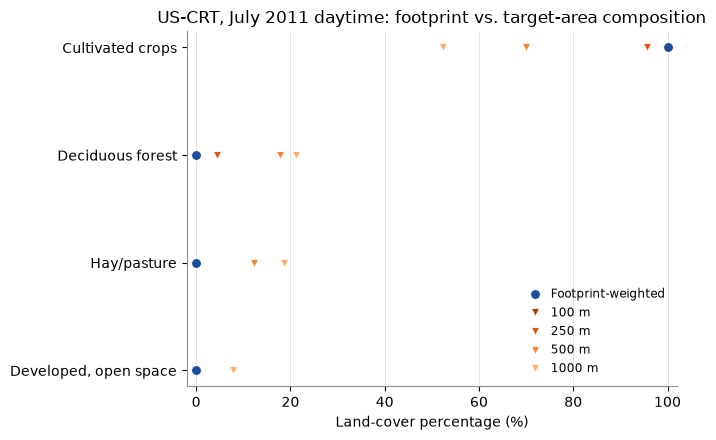
The filled circle is the footprint-weighted share, the triangles the target-area shares on a dark-to-light radius ramp. Crops sit at 100 % under the footprint and trail leftwards as the disc widens; every other class trails the other way, from 0 % under the footprint out to its share of the 1 km disc.

Figs. 1f and 6 — footprint against target-area values

daytime_pairs = periods.query("period == 'daytime'")

fig, ax = plot_footprint_target_scatter(daytime_pairs, variable="EVI")
ax.set_title("US-CRT daytime: matched monthly EVI, with the Eq. 7 RMA fits")
fig.tight_layout()

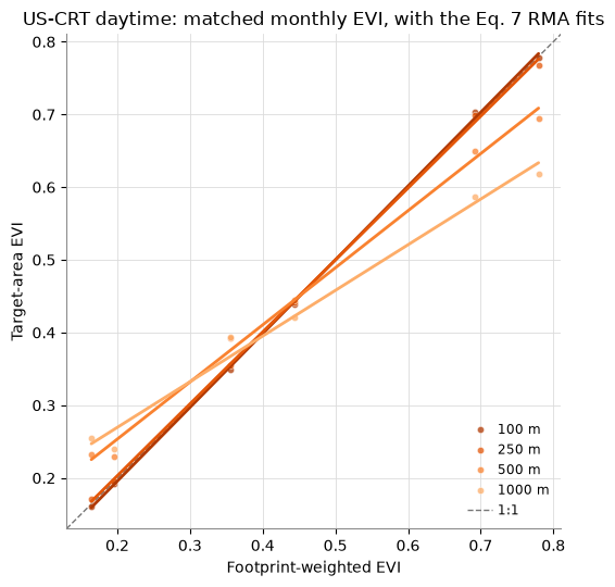
Six matched scenes per radius, under the reduced major axis fit of Eq. 7 and the 1:1 line. The 100 m series lies on 1:1; the wider discs pivot away from it, flattening exactly as their slopes in the table above say they should. The line is the RMA rather than ordinary least squares because both axes are spatial averages of one noisy raster and both carry error — an OLS slope would sit systematically shallower than the values the paper’s Table 1 reports.

Fig. 7 — density of the sensor location bias

fig, ax = plot_bias_density(daytime_pairs, threshold=BIAS_THRESHOLD)
ax.set_title("US-CRT daytime: sensor location bias (Eq. 6) by target area")
fig.tight_layout()

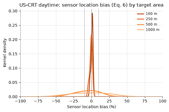
One Gaussian kernel density per radius over the per-scene biases. The peak is tall and narrow at 100 m and collapses into a broad, flat spread by 1000 m — the paper’s Fig. 7 result, that the wider the disc, the further a given month’s footprint-weighted value strays from it. The dashed guides are the ±10 % of BIAS_THRESHOLD; the published figure draws no guides, so they are opt-in.

Figs. 5 and 8 — the three-level index across target areas

site_levels = results.query("scope == 'site'").reset_index()

fig, ax = plot_level_bars(site_levels, level_column="level")
ax.set_ylabel("Percentage of evaluations (%)")
ax.set_title("US-CRT: representativeness level by target area")
fig.tight_layout()

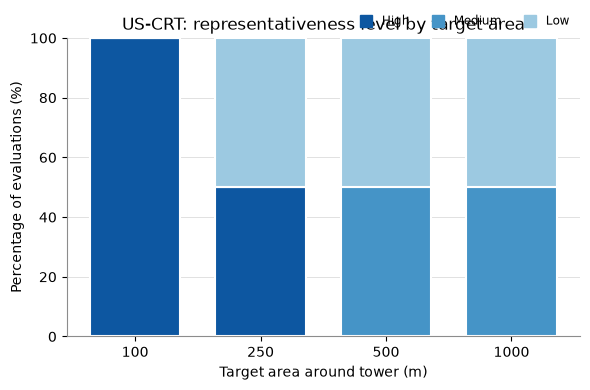
In the paper this panel pools hundreds of sites, and each bar is the share of sites still classified high at that radius. Here there is one site, so the bar pools its eight site-level verdicts instead — land cover and vegetation index, daytime and nighttime. The shape is the paper’s all the same: wholly high at 100 m, and progressively less so as the disc widens.

5. Exporting in the published layouts

representativeness_table reshapes the tidy frame into the column schema of the authors’ Datasets S4–S6, so a local analysis can be read next to, or concatenated with, the published tables. export_representativeness_tables writes all three to CSV in one call.

representativeness_table(results, "S6").round(3)

	SITE_ID	PERIOD	TARGET_AREA	VARIABLE	N	INTERCEPT	INTERCEPT_LCL	INTERCEPT_UCL	SLOPE	SLOPE_LCL	SLOPE_UCL	R2	RMSE	MAE	REP_EVI
0	US-CRT	daytime	100.0	EVI	6	-0.007	-0.021	0.006	1.014	0.984	1.046	1.000	0.006	0.005	high
1	US-CRT	daytime	250.0	EVI	6	0.005	-0.010	0.020	0.989	0.955	1.024	0.999	0.006	0.005	high
2	US-CRT	daytime	500.0	EVI	6	0.096	0.060	0.129	0.785	0.710	0.868	0.995	0.052	0.045	medium
3	US-CRT	daytime	1000.0	EVI	6	0.144	0.095	0.185	0.628	0.534	0.739	0.986	0.091	0.077	medium
4	US-CRT	nighttime	100.0	EVI	6	-0.009	-0.023	0.004	1.017	0.987	1.047	1.000	0.007	0.006	high
5	US-CRT	nighttime	250.0	EVI	6	0.003	-0.012	0.018	0.991	0.957	1.026	0.999	0.006	0.004	high
6	US-CRT	nighttime	500.0	EVI	6	0.095	0.058	0.128	0.787	0.712	0.870	0.995	0.051	0.044	medium
7	US-CRT	nighttime	1000.0	EVI	6	0.143	0.094	0.184	0.629	0.535	0.741	0.986	0.091	0.077	medium

What to take away

• The footprint is not the target area, and the gap is a function of radius. At US-CRT the tower represents its own 100 m surroundings almost perfectly and a 1 km cell only loosely — worth knowing before the site is used to validate a kilometre-scale product.

• Both evaluations agree on the direction and disagree on the pace. The categorical index falls off a cliff at 250 m because the chi-square test is sharpened by the fine grid; the continuous index degrades gradually. Read them together, and read the p-value with the grid in mind.

• The slope of Eq. 7 is the most informative single number here. A slope below one says the tower’s field swings more than the surrounding cell does, which is what upscaling from this site would have to correct for.

• The land-cover and EVI products here are synthetic. Swap in fetch_nlcd and fetch_landsat_evi, or any pair of rasters on disc, and nothing else in the notebook changes.

Next

• Footprint representativeness — the theory, all seven equations, and the classification tables.

• Validation against Chu et al. (2021) — these metrics recomputed from the authors’ own published climatology rasters.