Background

Author: Paul Inkenbrandt Date: 8/9/2026

Purpose: Compare footprint climatologies produced by the different flux-footprint models available in fluxfootprints — the Kljun et al. xarray rewrite (ffp_xr), the classic Kljun FFP port (ffp), the analytical Kormann & Meixner (2001) solution (km), a backward Lagrangian Stochastic model (ls), and the Wang et al. (2006) convective model (wang) — for the same station, meteorological inputs, and spatial domain.

This notebook reuses the data-loading and aerodynamic-parameter setup from footprint_workflow_example.ipynb, then diverges: instead of looping over months with a single model, it runs every model over one short comparison window and lines the results up on a common grid so they can be compared directly.

A few things that make a multi-model comparison harder than a single-model run:

• Grids don’t naturally line up. ffp, ffp_xr, and km build their grid from np.arange(domain_min, domain_max + dx, dx), so they match the requested DOMAIN/DX/DY exactly. ls bins particles into a histogram and reports bin centers (offset by half a cell), and wang builds its x axis outward from 0 before reflecting it, so its extent can differ slightly from the requested domain. Every model’s output is therefore re-gridded (xarray.DataArray.interp) onto one common (x, y) grid before any comparison is made.

• Not every model exposes a per-timestep footprint. ffp and ffp_xr expose both a per-timestep f_2d (used by the daily/monthly summarize_periods workflow in the other notebook) and a time-averaged fclim_2d. km, ls, and wang only expose fclim_2d. This notebook standardizes on model.get_footprint_climatology(), which every model implements, so the comparison is simply “run each model once on the same short window.”

• ``wang`` only runs for unstable (convective) conditions (ol < 0) and drops every other row internally, and ``ls`` is a Monte-Carlo model whose cost scales with n_particles x n_timesteps. Both are reasons to keep the comparison window short — this notebook uses a handful of midday timesteps from a single day rather than a full month.

Parameters and Libraries

# parameters to change or review for each run
STATIONID = 'US-UTW'
STATION_LAT  = 39.4452
STATION_LON  = -110.7287

# Comparison window: kept short on purpose (see Background) because the Lagrangian
# Stochastic model is Monte-Carlo (cost ~ n_particles * n_timesteps) and the Wang
# model needs unstable (ol < 0) daytime conditions to have any valid rows at all.
# Widen this once you know how long ls/wang take to run on your own data.
COMPARE_START = "2021-06-15 10:00"
COMPARE_END   = "2021-07-15 14:00"

DX, DY = 10.0, 10.0    # output raster resolution [m]
DOMAIN = (-600.0, 600.0, -600.0, 600.0)

MODEL_TYPES = ["ffp_xr", "ffp", "km", "ls", "wang"]
MODEL_LABELS = {
    "ffp_xr": "FFP (xarray)",
    "ffp":    "FFP (classic)",
    "km":     "Kormann-Meixner",
    "ls":     "Lagrangian Stochastic",
    "wang":   "Wang et al. (2006)",
}
# Okabe-Ito colorblind-safe palette, one fixed color per model (used in every chart below)
MODEL_COLORS = {
    "ffp_xr": "#0072B2",
    "ffp":    "#E69F00",
    "km":     "#009E73",
    "ls":     "#D55E00",
    "wang":   "#56B4E9",
}

REFERENCE_MODEL = "ffp_xr"   # what the difference maps / metrics are measured against

LS_N_PARTICLES = 5000   # reduced from the ls_footprint_adapter default (20000) to keep this demo fast

# path to input, following the same convention as footprint_workflow_example.ipynb
DAT_PATH = f'input_data/{STATIONID}_footprint.parquet'

import warnings
warnings.filterwarnings("ignore")

import time
import numpy as np
import pandas as pd
import matplotlib.pyplot as plt

import sys
sys.path.append("../../src")
from fluxfootprints.ffp_daily_monthly_helper import (
    build_climatology,
    compute_aerodynamic_params,
)

Read in Data and Prepare Aerodynamic Parameters

• Read in eddy covariance data file and create datetime index for start of record

• Compute aerodynamic parameters (z0 and zm), which every model below needs

# read in data and update to datetime_start index
df_all = pd.read_parquet(DAT_PATH)
df_all = df_all.sort_index()

# compute z0 and zm (needed by every model below)
df_all = compute_aerodynamic_params(
    df_all,
    inst_height='measurement_height',
    crop_height='crop_height_m',
    veg_type='alfalfa',
)

print(df_all.first_valid_index(), df_all.last_valid_index())

2021-06-01 00:00:00 2021-12-31 23:30:00

Select a Comparison Window

Subset to COMPARE_START–COMPARE_END and drop rows missing any field required across the five models. wang additionally needs some of those rows to be unstable (mo_length_1_1_1 < 0); the count is reported below so a failure further down is easy to diagnose.

# superset of columns needed across ffp / ffp_xr / km / ls / wang
REQ_FIELDS = ["mo_length_1_1_1", "v_sigma_1_1_1", "ustar_1_1_1", "wd_1_1_1", "ws_1_1_1", "zm", "z0"]

df_window = df_all.loc[COMPARE_START:COMPARE_END].copy()
df_window = df_window.dropna(subset=REQ_FIELDS)

n_unstable = int((df_window["mo_length_1_1_1"] < 0).sum())
print(f"Comparison window {COMPARE_START} -> {COMPARE_END}: {len(df_window)} valid timesteps "
      f"({n_unstable} unstable/convective, required by the wang model)")

assert len(df_window) > 0, "No valid timesteps in the comparison window - widen COMPARE_START/COMPARE_END"
df_window[REQ_FIELDS]

Comparison window 2021-06-15 10:00 -> 2021-07-15 14:00: 496 valid timesteps (161 unstable/convective, required by the wang model)

	mo_length_1_1_1	v_sigma_1_1_1	ustar_1_1_1	wd_1_1_1	ws_1_1_1	zm	z0
datetime_start
2021-07-05 06:30:00	16.47745	0.507604	0.222971	317.8547	3.111619	2.8923	0.03813
2021-07-05 07:00:00	76.45846	0.845518	0.384803	304.4949	4.991240	2.8923	0.03813
2021-07-05 07:30:00	67.52245	0.896419	0.372255	306.0229	5.067852	2.8923	0.03813
2021-07-05 08:00:00	73.47021	1.156355	0.461377	282.6653	6.251216	2.8923	0.03813
2021-07-05 08:30:00	40.42930	1.193933	0.341524	284.8635	5.399969	2.8923	0.03813
...	...	...	...	...	...	...	...
2021-07-15 12:00:00	-41.76294	1.342096	0.320913	196.9893	2.203942	2.8253	0.05043
2021-07-15 12:30:00	-24.65554	0.919386	0.261739	222.2221	1.442072	2.8253	0.05043
2021-07-15 13:00:00	-43.22299	0.827825	0.219982	180.3062	1.789526	2.8253	0.05043
2021-07-15 13:30:00	-35.05715	0.961006	0.236793	161.6139	1.865568	2.8253	0.05043
2021-07-15 14:00:00	-43.84708	1.262919	0.226805	157.1898	1.983701	2.8253	0.05043

496 rows × 7 columns

Run Every Footprint Model

Same build_climatology call as the main workflow notebook, just looped over MODEL_TYPES with the same column mapping and domain for every model. Failures (e.g. wang finding no unstable rows in the window) are caught and reported rather than stopping the notebook, so the comparison below just uses whichever models succeeded.

models = {}     # model_type -> fitted model instance
run_info = []   # per-model bookkeeping for the summary table

for model_type in MODEL_TYPES:
    label = MODEL_LABELS[model_type]
    print(f"Running {label} ({model_type}) ... ", end="", flush=True)

    model_kwargs = {"n_particles": LS_N_PARTICLES} if model_type == "ls" else {}

    t0 = time.perf_counter()
    try:
        model = build_climatology(
            df_window,
            model_type=model_type,
            ustar='ustar_1_1_1',
            ol='mo_length_1_1_1',
            umean='ws_1_1_1',
            sigmav='v_sigma_1_1_1',
            wind_dir='wd_1_1_1',
            zm='zm',
            z0='z0',
            h=2000.0,
            dx=DX,
            dy=DY,
            domain=DOMAIN,
            verbosity=0,   # quiet: default verbosity=2 logs every timestep, noisy across 5 models
            **model_kwargs,
        )
        runtime_s = time.perf_counter() - t0

        n_used = getattr(model, "ts_len", None)
        if n_used is None:
            n_used = model.results.attrs.get("n_timesteps", len(model.df))

        models[model_type] = model
        run_info.append({"model": model_type, "label": label, "status": "ok",
                          "n_timesteps": n_used, "runtime_s": runtime_s})
        print(f"done ({n_used} timesteps, {runtime_s:.1f}s)")

    except Exception as exc:
        runtime_s = time.perf_counter() - t0
        run_info.append({"model": model_type, "label": label, "status": f"failed: {exc}",
                          "n_timesteps": 0, "runtime_s": runtime_s})
        print(f"FAILED: {exc}")

run_df = pd.DataFrame(run_info)
run_df

Running FFP (xarray) (ffp_xr) ...

131/496 timesteps excluded due to range bounds or missing both z0 and umean.

done (365 timesteps, 1.3s)
Running FFP (classic) (ffp) ... done (365 timesteps, 1.5s)
Running Kormann-Meixner (km) ... done (496 timesteps, 130.8s)
Running Lagrangian Stochastic (ls) ... done (496 timesteps, 637.9s)
Running Wang et al. (2006) (wang) ... done (161 timesteps, 0.0s)

	model	label	status	n_timesteps	runtime_s
0	ffp_xr	FFP (xarray)	ok	365	1.259231
1	ffp	FFP (classic)	ok	365	1.487458
2	km	Kormann-Meixner	ok	496	130.835229
3	ls	Lagrangian Stochastic	ok	496	637.911606
4	wang	Wang et al. (2006)	ok	161	0.035872

Regrid Every Model onto a Common Grid

Every model exposes get_footprint_climatology() (dims x, y), but on its own native grid (see Background). xarray.interp puts each one onto the same common_x/common_y grid built from DOMAIN/DX/DY; models whose native grid already matches that (ffp, ffp_xr, km) pass through essentially unchanged. Interpolating outside a model’s native extent fills with 0, which can shave a little mass off the total — mainly for ls and wang — so each raster is renormalized to integrate to 1 over the common grid afterward. Treat shape and peak-location differences as the meaningful signal here; absolute density right at the domain edges is the part most affected by this step.

common_x = np.arange(DOMAIN[0], DOMAIN[1] + DX, DX)
common_y = np.arange(DOMAIN[2], DOMAIN[3] + DY, DY)
cell_area = DX * DY

rasters = {}   # model_type -> 2D numpy array (nx, ny) on the common grid, sum*cell_area == 1

for model_type, model in models.items():
    fclim = model.get_footprint_climatology().transpose("x", "y")   # native grid
    regridded = fclim.interp(x=common_x, y=common_y, method="linear",
                              kwargs={"fill_value": 0.0}).fillna(0.0)

    arr = np.clip(regridded.values, 0.0, None)   # interpolation can create tiny negative ripples
    total = arr.sum() * cell_area
    if total > 0:
        arr = arr / total
    rasters[model_type] = arr

print(f"Common grid: {len(common_x)} x {len(common_y)} cells at {DX}m x {DY}m")

Common grid: 121 x 121 cells at 10.0m x 10.0m

Side-by-Side Footprint Maps

vmax = max(arr.max() for arr in rasters.values())

fig, axes = plt.subplots(1, len(rasters), figsize=(4.2 * len(rasters), 4.2), squeeze=False)
axes = axes[0]

for ax, model_type in zip(axes, rasters):
    im = ax.pcolormesh(common_x, common_y, rasters[model_type].T, cmap="viridis",
                        vmin=0, vmax=vmax, shading="auto")
    ax.plot(0, 0, marker="^", color="white", markeredgecolor="black", markersize=9, zorder=5)
    ax.set_title(MODEL_LABELS[model_type])
    ax.set_xlabel("x [m]")
    ax.set_aspect("equal")

axes[0].set_ylabel("y [m]")
fig.colorbar(im, ax=axes.tolist(), shrink=0.85, label="Footprint density [m$^{-2}$]")
fig.suptitle(f"{STATIONID} footprint climatology, {COMPARE_START} to {COMPARE_END}", y=1.03)
plt.show()

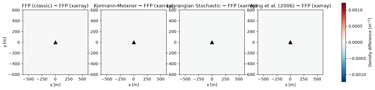
Difference Maps Relative to the Reference Model

REFERENCE_MODEL (set above, default ffp_xr) is subtracted from every other model’s raster. Red = that model predicts more source contribution than the reference at that cell; blue = less.

ref_arr = rasters[REFERENCE_MODEL]
other_types = [m for m in rasters if m != REFERENCE_MODEL]

diffs = {m: rasters[m] - ref_arr for m in other_types}
dmax = max(np.abs(d).max() for d in diffs.values())

fig, axes = plt.subplots(1, len(other_types), figsize=(4.2 * len(other_types), 4.2), squeeze=False)
axes = axes[0]

for ax, model_type in zip(axes, other_types):
    im = ax.pcolormesh(common_x, common_y, diffs[model_type].T, cmap="RdBu_r",
                        vmin=-dmax, vmax=dmax, shading="auto")
    ax.plot(0, 0, marker="^", color="black", markersize=9, zorder=5)
    ax.set_title(f"{MODEL_LABELS[model_type]} − {MODEL_LABELS[REFERENCE_MODEL]}")
    ax.set_xlabel("x [m]")
    ax.set_aspect("equal")

axes[0].set_ylabel("y [m]")
fig.colorbar(im, ax=axes.tolist(), shrink=0.85, label="Density difference [m$^{-2}$]")
plt.show()

Quantitative Comparison Metrics

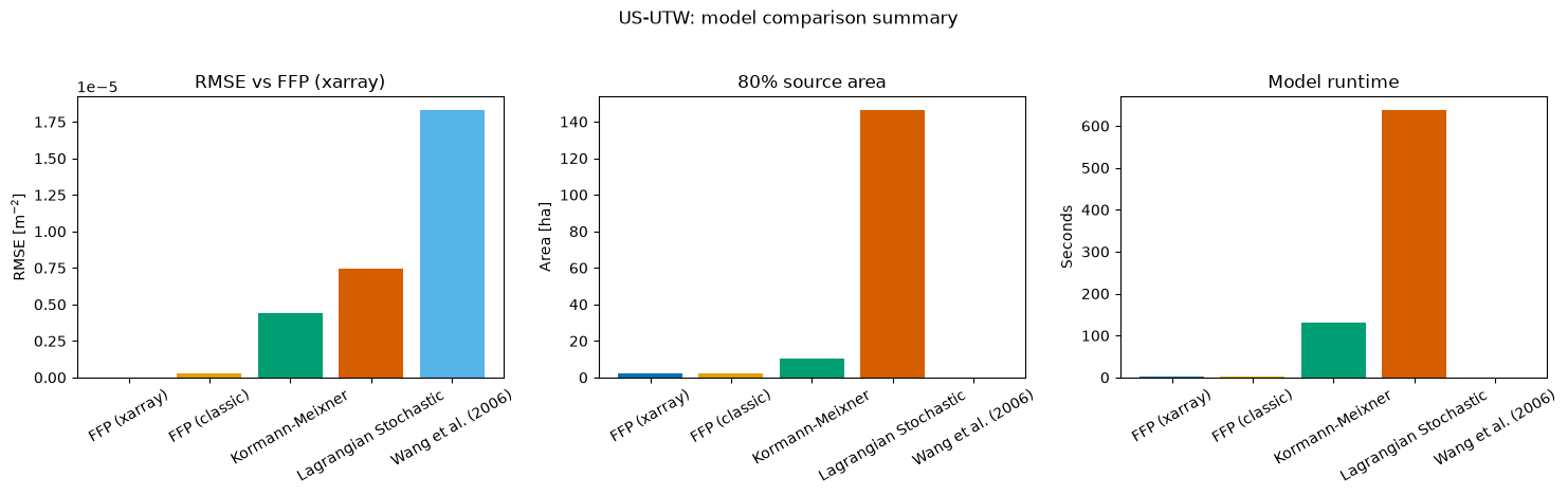
For each model, relative to REFERENCE_MODEL:

• RMSE_vs_ref — cell-by-cell root-mean-square difference in footprint density.

• peak_dist_m / peak_diff_vs_ref_m — distance from the tower to the model’s peak contribution cell, and how far that is from the reference model’s peak.

• overlap80_vs_ref_pct — percent overlap between the two models’ 80% source-area cells.

• source_area_80_ha — size of the model’s own 80% source area, in hectares.

• runtime_s — wall-clock time for build_climatology on this comparison window.

def peak_distance(arr, x, y):
    """Distance from the tower (0, 0) to the cell of maximum footprint density."""
    ix, iy = np.unravel_index(np.argmax(arr), arr.shape)
    return float(np.hypot(x[ix], y[iy]))

def mask_80(arr):
    """Boolean mask of the smallest set of cells containing 80% of the footprint."""
    flat = arr.flatten()
    order = np.argsort(flat)[::-1]
    cumsum = np.cumsum(flat[order]) * cell_area
    n80 = np.searchsorted(cumsum, 0.8)
    thresh = flat[order][min(n80, flat.size - 1)]
    return arr >= thresh

def source_area_80_ha(arr):
    return mask_80(arr).sum() * cell_area / 10_000.0

ref_mask80 = mask_80(ref_arr)
peak_ref = peak_distance(ref_arr, common_x, common_y)

metrics = []
for model_type, arr in rasters.items():
    peak = peak_distance(arr, common_x, common_y)
    overlap = float((mask_80(arr) & ref_mask80).sum() / ref_mask80.sum() * 100.0)
    runtime_s = run_df.loc[run_df["model"] == model_type, "runtime_s"].iloc[0]

    metrics.append({
        "model": MODEL_LABELS[model_type],
        "RMSE_vs_ref": float(np.sqrt(np.mean((arr - ref_arr) ** 2))),
        "peak_dist_m": peak,
        "peak_diff_vs_ref_m": abs(peak - peak_ref),
        "overlap80_vs_ref_pct": overlap,
        "source_area_80_ha": source_area_80_ha(arr),
        "runtime_s": runtime_s,
    })

metrics_df = pd.DataFrame(metrics).set_index("model")
metrics_df.round(3)

	RMSE_vs_ref	peak_dist_m	peak_diff_vs_ref_m	overlap80_vs_ref_pct	source_area_80_ha	runtime_s
model
FFP (xarray)	0.0	10.000	0.000	100.000	2.23	1.259
FFP (classic)	0.0	10.000	0.000	99.103	2.21	1.487
Kormann-Meixner	0.0	22.361	12.361	100.000	10.29	130.835
Lagrangian Stochastic	0.0	848.528	838.528	100.000	146.41	637.912
Wang et al. (2006)	0.0	10.000	0.000	4.484	0.10	0.036

Visual Summary of Metrics

plot_order = list(rasters.keys())
x_labels = [MODEL_LABELS[m] for m in plot_order]
bar_colors = [MODEL_COLORS[m] for m in plot_order]

fig, axes = plt.subplots(1, 3, figsize=(15, 4.5))

axes[0].bar(x_labels, metrics_df.loc[x_labels, "RMSE_vs_ref"], color=bar_colors)
axes[0].set_title(f"RMSE vs {MODEL_LABELS[REFERENCE_MODEL]}")
axes[0].set_ylabel("RMSE [m$^{-2}$]")

axes[1].bar(x_labels, metrics_df.loc[x_labels, "source_area_80_ha"], color=bar_colors)
axes[1].set_title("80% source area")
axes[1].set_ylabel("Area [ha]")

axes[2].bar(x_labels, metrics_df.loc[x_labels, "runtime_s"], color=bar_colors)
axes[2].set_title("Model runtime")
axes[2].set_ylabel("Seconds")

for ax in axes:
    ax.tick_params(axis="x", rotation=30)

fig.suptitle(f"{STATIONID}: model comparison summary", y=1.03)
fig.tight_layout()
plt.show()

Notes & Caveats

• The comparison window is intentionally short. Widen COMPARE_START/COMPARE_END for a more representative comparison, but check ls and wang runtimes in run_df first — ls cost scales with n_particles x n_timesteps.

• Regridding + renormalizing changes absolute densities, most for ls and wang whose native grids don’t match DOMAIN exactly. Shape and peak-location differences are more trustworthy than small density differences near the domain edges.

• ``wang`` silently uses fewer rows than the other models — it drops every timestep with ol >= 0 (stable/neutral) before running. If it’s missing from run_df entirely, the window had no unstable rows at all.

• ``ls`` is stochastic. Its raster will change slightly between runs; increase LS_N_PARTICLES (at the cost of runtime) if it looks noisy relative to the other models.

• Metrics are all relative to ``REFERENCE_MODEL``. Change it at the top of the notebook and rerun from “Regrid Every Model onto a Common Grid” onward to compare against a different baseline.

• This notebook does not export GeoTIFFs. For that, use the daily/monthly summarize_periods + export_rasters_geotiff workflow from footprint_workflow_example.ipynb (works for ffp/ffp_xr, which expose a per-timestep footprint), or call model.to_netcdf(path) on any individual model here to save its own climatology.