Getting Started: Wang (2006) Cross‑Wind Integrated Footprint

This notebook shows how to use the wang_footprint.py module from the fluxfootprints library to compute the Wang et al. (2006) cross‑wind‑integrated footprint, and (optionally) reconstruct a 2‑D footprint by assuming a Gaussian lateral spread.

What you’ll do

1. Import the Wang (2006) functions from your local src checkout.

2. Compute the 1‑D cross‑wind integrated footprint (f_y(x)).

3. (Optional) Reconstruct a 2‑D footprint (f(x, y)) and visualize it.

4. Extract practical distances (e.g., x for 50%, 80%, 90% cumulative contribution).

CBL validity: The Wang (2006) parameterisation targets convective daytime conditions and requires negative Monin‑Obukhov length L < 0. Use with caution outside the published range.

# --- Setup & Imports ----------------------------------------------------------
import os, sys, math, numpy as np

# Use your local project layout: notebook in e.g. `notebooks/`, package in `src/`
# The user requested: use sys.path.append("../../src")
sys.path.append("../../src")

# Now import from the package/module
from fluxfootprints.wang_footprint import wang2006_fy, reconstruct_gaussian_2d
print("Imports OK. Using fluxfootprints from:", [p for p in sys.path if p.endswith("/src")])

Imports OK. Using fluxfootprints from: ['../../src']

# --- Quick environment check --------------------------------------------------
import numpy as np, matplotlib
print("NumPy:", np.__version__)
print("Matplotlib:", matplotlib.__version__)

# Optional: show docstring summaries
print("\nwang2006_fy:", wang2006_fy.__doc__.splitlines()[0])
print("reconstruct_gaussian_2d:", reconstruct_gaussian_2d.__doc__.splitlines()[0])

NumPy: 2.2.2
Matplotlib: 3.10.0

wang2006_fy: Cross‑wind integrated footprint ``f_y(x)`` (m⁻¹).
reconstruct_gaussian_2d: Reconstruct a 2‑D footprint ``f(x,y)`` from a 1‑D ``f_y(x)``.

1) Provide inputs

You need:

• zm — measurement height above ground (m)

• h — convective boundary‑layer height (m)

• L — Monin‑Obukhov length (negative for convective)

• Optional: U (mean wind speed, m s⁻¹) and sigma_v (lateral velocity std, m s⁻¹) to define the lateral spread for the 2‑D reconstruction.

Below, the cell will try to discover any example CSV/JSON in a nearby examples/ or data/ folder. If none is found, it will fall back to a synthetic convective case that produces a reasonable footprint.

# --- Try to auto‑discover example inputs -------------------------------------
from pathlib import Path
import json, csv

def try_load_examples():
    candidates = [
        Path("../examples"), Path("../../examples"),
        Path("./examples"), Path("../data"), Path("../../data")
    ]
    # Simple heuristics: look for small CSV/JSON that might contain zm,h,L,U,sigma_v
    for base in candidates:
        if not base.exists():
            continue
        for ext in ("*.csv", "*.json"):
            for f in base.glob(ext):
                try:
                    if f.suffix.lower() == ".json":
                        with open(f, "r", encoding="utf-8") as fp:
                            data = json.load(fp)
                        keys = {k.lower() for k in data.keys()}
                        if {"zm","h","l"}.issubset(keys):
                            return dict(zm=float(data["zm"]), h=float(data["h"]), L=float(data["l"]),
                                        U=float(data.get("U", 3.5)), sigma_v=float(data.get("sigma_v", 0.6))), f
                    else:  # CSV
                        with open(f, "r", encoding="utf-8") as fp:
                            reader = csv.DictReader(fp)
                            for row in reader:
                                keys = {k.lower() for k in row.keys()}
                                if {"zm","h","l"}.issubset(keys):
                                    return dict(zm=float(row["zm"]), h=float(row["h"]), L=float(row["L"]),
                                                U=float(row.get("U", 3.5)), sigma_v=float(row.get("sigma_v", 0.6))), f
                except Exception:
                    # Not an expected format; keep scanning
                    pass
    return None, None

params, src_file = try_load_examples()

if params is None:
    # Fallback: synthetic daytime convective case
    params = dict(
        zm=3.0,     # m
        h=800.0,    # m
        L=-120.0,   # m  (must be negative for convective)
        U=3.5,      # m/s
        sigma_v=0.6 # m/s
    )
    print("No example file found. Using synthetic parameters:", params)
else:
    print(f"Loaded example parameters from {src_file}: {params}")

zm, h, L, U, sigma_v = params["zm"], params["h"], params["L"], params["U"], params["sigma_v"]
assert L < 0.0, "Wang (2006) requires convective conditions (L < 0)."

No example file found. Using synthetic parameters: {'zm': 3.0, 'h': 800.0, 'L': -120.0, 'U': 3.5, 'sigma_v': 0.6}

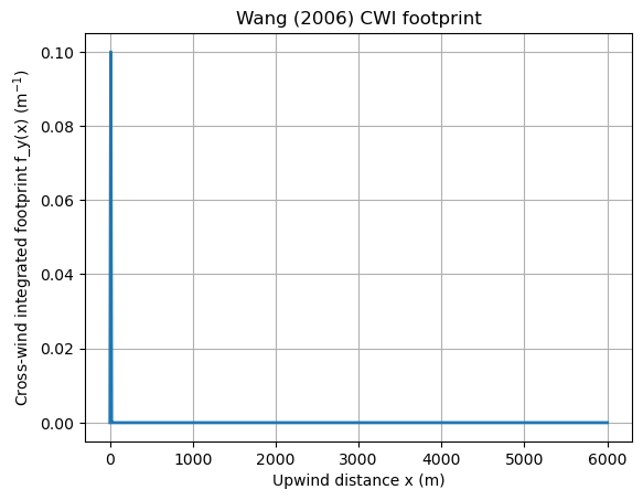
2) Compute the 1‑D cross‑wind‑integrated footprint (f_y(x))

We’ll evaluate (f_y(x)) along a stream‑wise distance vector x (positive upwind).

import numpy as np

# Stream‑wise grid (m); extend far enough upwind for the tail to decay
x = np.linspace(0.0, 6000.0, 601)  # 10 m spacing
fy = wang2006_fy(x, zm=zm, h=h, L=L)

# Basic checks
dx = x[1] - x[0]
mass = np.trapezoid(fy, x)
print(f"Integral ∫ f_y dx ≈ {mass:.6f} (should be ~1.0)")
print(f"Max f_y at x ≈ {x[np.argmax(fy)]:.1f} m")

Integral ∫ f_y dx ≈ 1.000000 (should be ~1.0)
Max f_y at x ≈ 10.0 m

# --- Plot f_y(x) --------------------------------------------------------------
import matplotlib.pyplot as plt

plt.figure()
plt.plot(x, fy, lw=2)
plt.xlabel("Upwind distance x (m)")
plt.ylabel("Cross-wind integrated footprint f_y(x) (m$^{-1}$)")
plt.title("Wang (2006) CWI footprint")
plt.grid(True)
plt.show()

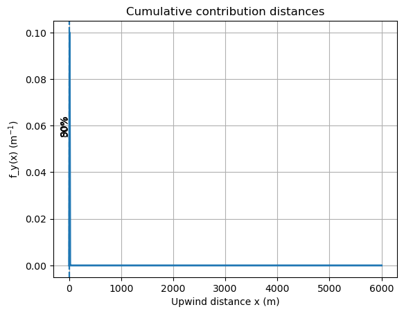
3) Practical distances by cumulative contribution

You can extract distances that capture a chosen fraction of the source area (e.g., 50%, 80%, 90%) by integrating (f_y(x)).

cum = np.cumsum(fy) * (x[1] - x[0])

def x_at_fraction(frac):
    idx = np.searchsorted(cum, frac)
    return float(x[min(idx, len(x)-1)])

x50, x80, x90 = x_at_fraction(0.50), x_at_fraction(0.80), x_at_fraction(0.90)
print(f"x_50% ≈ {x50:.1f} m,  x_80% ≈ {x80:.1f} m,  x_90% ≈ {x90:.1f} m")

x_50% ≈ 10.0 m,  x_80% ≈ 10.0 m,  x_90% ≈ 10.0 m

# Re-plot with markers for 50/80/90%
import matplotlib.pyplot as plt

plt.figure()
plt.plot(x, fy, lw=2)
for xv, label in [(x50, "50%"), (x80, "80%"), (x90, "90%")]:
    plt.axvline(x=xv, ls="--")
    plt.text(xv, max(fy)*0.6, label, rotation=90, va="center", ha="right")
plt.xlabel("Upwind distance x (m)")
plt.ylabel("f_y(x) (m$^{-1}$)")
plt.title("Cumulative contribution distances")
plt.grid(True)
plt.show()

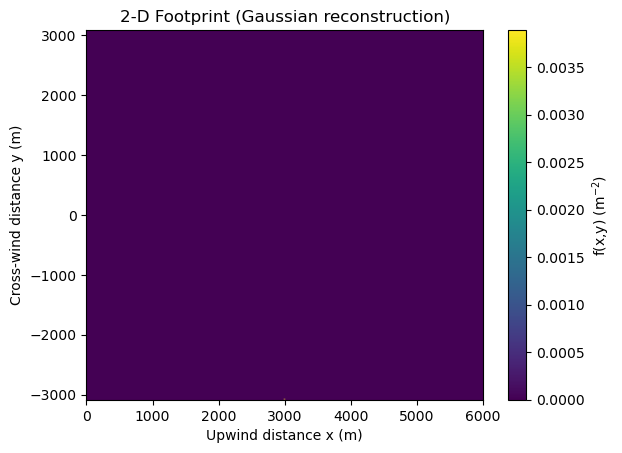
4) (Optional) Reconstruct a 2‑D footprint (f(x, y))

Use a Gaussian lateral distribution with width (\sigma_y(x)). By default, (\sigma_y = \alpha `x) with (:nbsphinx-math:alpha :nbsphinx-math:approx 0.3`). If you have turbulence stats, you can pass sigma_v and U to use (\sigma_y = (\sigma_v/U),x).

# Compute the 2-D reconstruction using turbulence-based sigma_y
X, Y, F = reconstruct_gaussian_2d(x, fy, sigma_v=sigma_v, U=U, ny=241)

# Sanity check: F integrates to ~1 over the domain
dx = x[1] - x[0]
dy = Y[1,0] - Y[0,0]
mass2d = np.sum(F * dx * dy)
print(f"Double integral ∬ F dx dy ≈ {mass2d:.6f}")

Double integral ∬ F dx dy ≈ 1.000000

# --- Visualize the 2-D footprint ---------------------------------------------
import matplotlib.pyplot as plt
extent = [x.min(), x.max(), Y.min(), Y.max()]

plt.figure()
plt.imshow(F.T, origin="lower", aspect="auto", extent=extent)
plt.colorbar(label="f(x,y) (m$^{-2}$)")
plt.xlabel("Upwind distance x (m)")
plt.ylabel("Cross-wind distance y (m)")
plt.title("2-D Footprint (Gaussian reconstruction)")
plt.show()

5) Save results

These examples show how to export the computed arrays to common formats.

# Save 1-D footprint to CSV
import pandas as pd
one_d = pd.DataFrame({"x_m": x, "f_y_per_m": fy, "cum_frac": np.cumsum(fy)*(x[1]-x[0])})
one_d.to_csv("wang2006_fy_example.csv", index=False)
print("Wrote: wang2006_fy_example.csv")

# Save 2-D footprint as NumPy .npz
np.savez_compressed("wang2006_2d_example.npz", X=X, Y=Y, F=F)
print("Wrote: wang2006_2d_example.npz")

Wrote: wang2006_fy_example.csv
Wrote: wang2006_2d_example.npz

Troubleshooting

• ``ValueError: L must be negative`` — The Wang (2006) scheme is for convective conditions; ensure your L is negative.

• ``x must be non‑negative`` — The model expects positive upwind distances (start at x=0 and move upstream).

• If your ∫ f_y dx or ∬ F dx dy is not close to 1, ensure your x range is sufficiently long so the tail has decayed.

• If you don’t have sigma_v and U, omit them; the model will use a simple (\sigma_y = \alpha `x) with ``alpha=0.3` by default.

Next steps

• Combine the 2‑D footprint with gridded surface properties (land cover, LAI, NDVI) to compute weighted footprints.

• Convert the 2‑D grid to geospatial rasters (GeoTIFF) or vector contours (GeoPackage) using your GIS stack.

• Batch‑process multiple time periods and summarise daily or monthly contributions using your preferred data pipeline.