Getting Started: Lagrangian Stochastic (LS) Footprint Model

This notebook shows how to use the ``ls_footprint_model.py`` module to compute a simple 2‑D flux footprint from eddy‑covariance tower data. It uses the attached example configuration (US-UTE.ini) and data file referenced therein.

1) Setup

This section adjusts sys.path so you can import from your local source tree, then imports the LS model. If you’ve installed the package, the first import will also work.

# --- Standard library
import os, sys, math, pathlib, warnings

# --- Third‑party
import numpy as np
import pandas as pd
import matplotlib.pyplot as plt

sys.path.append("../../src")
from fluxfootprints.ls_footprint_model import LSFootprintConfig, BackwardLSModel

plt.rcParams["figure.dpi"] = 120
warnings.filterwarnings("ignore")
print("Imports ready.")

Imports ready.

2) Load site configuration and data

We read US-UTE.ini to discover the time column, wind variables, and file names. Then we load the CSV it references and make a minimal set of variables needed by the LS model.

import configparser
from pathlib import Path

# Point to the example INI and CSV (adjust paths as needed)
ini_path = Path("US-UTE.ini")
if not ini_path.exists():
    ini_path = Path("./input_data/US-UTE.ini")  # fallback for this shared environment

cfg = configparser.ConfigParser(interpolation=None)
cfg.read(ini_path)

# Pull the essentials
date_col = cfg.get("DATA", "datestring_col")
date_fmt = cfg.get("METADATA", "date_parser")
skiprows = cfg.getint("METADATA", "skiprows", fallback=0)
missing_val = cfg.getfloat("METADATA", "missing_data_value", fallback=-9999.0)

# Columns for wind speed and direction
ws_col = cfg.get("DATA", "wind_spd_col", fallback="WS")
wd_col = cfg.get("DATA", "wind_dir_col", fallback="WD")

# Resolve the climate/data CSV next to the INI, or in the same folder
csv_rel = cfg.get("METADATA", "climate_file_path")
csv_path = ini_path.parent / csv_rel
if not csv_path.exists():
    csv_path = Path("/mnt/data") / csv_rel  # fallback

# Load data
parse = lambda s: pd.to_datetime(s, format=date_fmt, errors="coerce")
df = pd.read_csv(csv_path, skiprows=skiprows)
df[date_col] = df[date_col].apply(parse)
df = df.dropna(subset=[date_col]).set_index(date_col).sort_index()

# Basic cleaning for common missing value flags
df = df.replace({missing_val: np.nan, -9999: np.nan, -9999.0: np.nan})

print(f"Loaded {len(df):,} rows from:", csv_path)
df.head()

Loaded 3,283 rows from: input_data/US-UTE_HH_202406241430_202409251400.csv

	datetime_start	TIMESTAMP_END	CO2	CO2_SIGMA	H2O	H2O_SIGMA	FC	FC_SSITC_TEST	LE	LE_SSITC_TEST	...	TA_1_2_1	RH_1_2_1	T_DP_1_2_1	TA_1_3_1	RH_1_3_1	T_DP_1_3_1	TA_1_4_1	PBLH_F	TS_2_1_1	SWC_2_1_1
TIMESTAMP_START
2024-06-24 14:30:00	2024-06-24 14:30:00	202406241500	427.0199	0.628133	17.26862	1.019290	0.069210	NaN	156.40850	NaN	...	29.95141	33.26877	12.052600	30.32464	33.45364	12.46181	30.06976	1665.4670	25.72815	22.44161
2024-06-24 15:00:00	2024-06-24 15:00:00	202406241530	425.9499	1.019297	15.18936	0.703052	0.285446	NaN	138.30920	NaN	...	30.02516	29.22197	10.155240	30.35956	29.77183	10.72635	30.13765	1765.9350	25.52736	22.41975
2024-06-24 15:30:00	2024-06-24 15:30:00	202406241600	426.4163	1.965228	14.87533	0.808026	1.081928	NaN	154.11530	NaN	...	30.24634	28.28498	9.838229	30.69433	28.63222	10.41335	30.40344	1495.7350	25.12511	22.32785
2024-06-24 16:00:00	2024-06-24 16:00:00	202406241630	426.0534	2.665907	15.61140	1.002919	0.519664	NaN	135.56180	NaN	...	30.75179	28.75255	10.538220	31.14621	29.16225	11.09066	30.90061	1491.0620	24.63557	22.18172
2024-06-24 16:30:00	2024-06-24 16:30:00	202406241700	427.8476	1.102921	15.21034	0.703084	1.147608	NaN	95.06287	NaN	...	29.16274	30.77158	10.165810	29.57434	30.96792	10.63069	29.30510	341.9711	24.14865	22.03216

5 rows × 61 columns

3) Choose a time slice and prepare LS model inputs

The LS model needs:

• zm (receptor height, m)

• ustar (friction velocity, m s⁻¹)

• L (Monin–Obukhov length, m) — not used in this minimal implementation but kept for extension

• h (boundary‑layer height, m)

• wind_dir_deg (meteorological from direction, degrees)

• surface roughness z0 and a numerical grid/domain

If your dataset has a USTAR column, we use that. Otherwise we estimate (u_*) from wind speed by the neutral log‑law (requires assumptions for zm and z0).

KAPPA = 0.4

# Assumptions you can tune for your site
zm_default = 4.0   # receptor height [m]
z0_default = 0.1   # roughness length [m]
h_default  = 1000.0
L_default  = -50.0  # kept for API compatibility; not used in the core model

# Pick a representative timestamp with non‑missing wind + speed
needed = [wd_col]
if "USTAR" in df.columns:
    needed.append("USTAR")
else:
    needed.append(ws_col)

sub = df.dropna(subset=needed).copy()
if sub.empty:
    raise RuntimeError("No rows with required variables present. Check column names and missing values.")

row = sub.iloc[0]  # take the first valid row; feel free to select by date/time

# Derive ustar if needed
if "USTAR" in df.columns and pd.notna(row.get("USTAR")):
    ustar = float(row["USTAR"])
else:
    # Estimate u* with neutral log profile: u* = κ U / ln(zm / z0)
    U = float(row[ws_col])
    ustar = KAPPA * U / math.log(zm_default / z0_default)

wind_dir_deg = float(row[wd_col])
zm, z0, h, L = zm_default, z0_default, h_default, L_default

print(f"Selected time: {row.name}")
print(f"u* = {ustar:.3f} m s⁻1 | wind_dir = {wind_dir_deg:.1f}° | zm={zm} m, z0={z0} m, h={h} m")

Selected time: 2024-06-24 14:30:00
u* = 0.285 m s⁻1 | wind_dir = 83.8° | zm=4.0 m, z0=0.1 m, h=1000.0 m

4) Run the model

cfg = LSFootprintConfig(
    zm=zm,
    ustar=ustar,
    L=L,
    h=h,
    wind_dir_deg=wind_dir_deg,
    z0=z0,
    n_particles=20_000,   # increase for smoother fields
    dt=0.25,
    t_max=600.0,
    domain=(2000.0, 2000.0),
    dx=20.0,
    dy=20.0,
    seed=42,              # reproducible runs
)
model = BackwardLSModel(cfg)
model.run()

x, y, F = model.footprint()
xx, fx = model.crosswind_integrated()

F.min(), F.max(), F.sum()

(np.float64(0.0), np.float64(0.00039797840676442895), np.float64(0.0025))

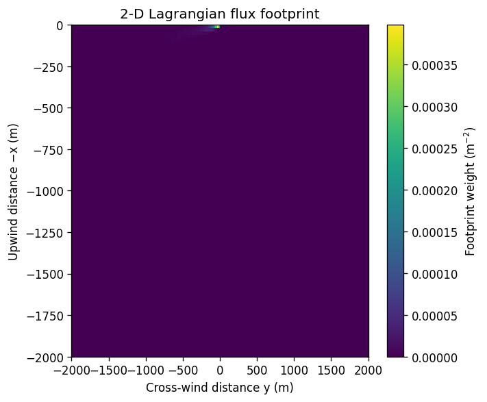
5) Visualize the footprint

plt.figure(figsize=(6, 5))
plt.pcolormesh(y, x, F, shading="auto")
plt.colorbar(label="Footprint weight (m$^{-2}$)")
plt.xlabel("Cross‑wind distance y (m)")
plt.ylabel("Upwind distance −x (m)")
plt.title("2‑D Lagrangian flux footprint")
plt.tight_layout()
plt.show()

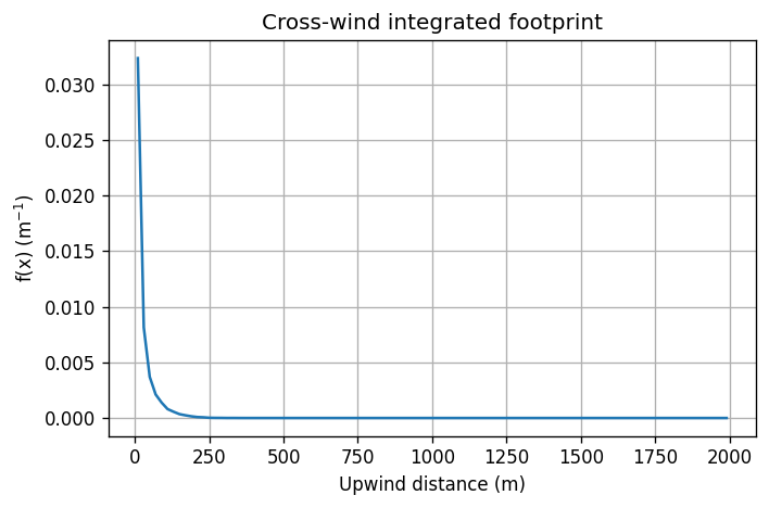
plt.figure(figsize=(6, 4))
plt.plot(-xx, fx)  # positive axis for downwind distance
plt.xlabel("Upwind distance (m)")
plt.ylabel("f(x) (m$^{-1}$)")
plt.title("Cross‑wind integrated footprint")
plt.grid(True)
plt.tight_layout()
plt.show()

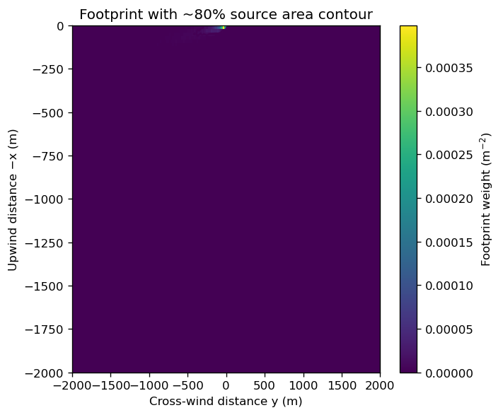
6) Optional: 80% source area contour

Below we compute a density threshold such that the integral of the footprint inside the contour is ~80% of the total. We then plot that as a single contour line.

# Convert density (m^-2) to probability mass per cell
cell_mass = F * cfg.dx * cfg.dy
flat = cell_mass.ravel()
order = np.argsort(flat)[::-1]
csum = np.cumsum(flat[order])

# Find threshold where cumulative mass first exceeds 0.8
idx_thr = int(np.searchsorted(csum, 0.8))
thr_mass = flat[order][idx_thr]
thr_density = thr_mass / (cfg.dx * cfg.dy)

plt.figure(figsize=(6, 5))
plt.pcolormesh(y, x, F, shading="auto")
plt.colorbar(label="Footprint weight (m$^{-2}$)")
cc = plt.contour(y, x, F, levels=[thr_density])
plt.clabel(cc, fmt="80% area", inline=True, fontsize=8)
plt.xlabel("Cross‑wind distance y (m)")
plt.ylabel("Upwind distance −x (m)")
plt.title("Footprint with ~80% source area contour")
plt.tight_layout()
plt.show()

7) Save outputs (optional)

out_dir = Path("outputs")
out_dir.mkdir(exist_ok=True)

# Save grids
np.save(out_dir / "footprint_density.npy", F)
np.savetxt(out_dir / "footprint_density.csv", F, delimiter=",")
np.savetxt(out_dir / "x_centers_m.csv", x, delimiter=",")
np.savetxt(out_dir / "y_centers_m.csv", y, delimiter=",")

# Save figures
plt.figure(figsize=(6, 5))
plt.pcolormesh(y, x, F, shading="auto")
plt.colorbar(label="Footprint weight (m$^{-2}$)")
plt.xlabel("Cross‑wind distance y (m)")
plt.ylabel("Upwind distance −x (m)")
plt.title("2‑D LS Footprint")
plt.tight_layout()
plt.savefig(out_dir / "footprint_2d.png", dpi=200)
plt.close()

plt.figure(figsize=(6, 4))
plt.plot(-xx, fx)
plt.xlabel("Upwind distance (m)")
plt.ylabel("f(x) (m$^{-1}$)")
plt.title("Cross‑wind integrated footprint")
plt.grid(True)
plt.tight_layout()
plt.savefig(out_dir / "footprint_fx.png", dpi=200)
plt.close()

print("Saved outputs to:", out_dir.resolve())

8) Tips & next steps

• Increase n_particles for smoother fields (e.g., 50,000–200,000).

• Adjust domain, dx and dy to control the spatial extent and resolution.

• If you have measured USTAR, use it directly; otherwise, provide a better local estimate for z0 and set your actual zm.

• The current L parameter is kept for future extensions (e.g., stability‑dependent turbulence); it is not used in the core update step here.

• For climatological footprints, repeat runs across many time steps and average the resulting F fields (watch memory and runtime).